星晴

无标签

发布日期: 2019-11-26

阅读次数:

Python 3

Seaborn 数据可视化基础

介绍

Matplotlib 是支持 Python 语言的开源绘图库，因为其支持丰富的绘图类型、简单的绘图方式以及完善的接口文档，深受 Python 工程师、科研学者、数据工程师等各类人士的喜欢。Seaborn 是以 Matplotlib 为核心的高阶绘图库，无需经过复杂的自定义即可绘制出更加漂亮的图形，非常适合用于数据可视化探索。

知识点

关联图
类别图
分布图
回归图
矩阵图
组合图

Seaborn 介绍

Matplotlib 应该是基于 Python 语言最优秀的绘图库了，但是它也有一个十分令人头疼的问题，那就是太过于复杂了。3000 多页的官方文档，上千个方法以及数万个参数，属于典型的你可以用它做任何事，但又无从下手。尤其是，当你想通过 Matplotlib 调出非常漂亮的效果时，往往会伤透脑筋，非常麻烦。

Seaborn 基于 Matplotlib 核心库进行了更高阶的 API 封装，可以让你轻松地画出更漂亮的图形。Seaborn 的漂亮主要体现在配色更加舒服、以及图形元素的样式更加细腻，下面是 Seaborn 官方给出的参考图。

Seaborn 具有如下特点：

内置数个经过优化的样式效果。
增加调色板工具，可以很方便地为数据搭配颜色。
单变量和双变量分布绘图更为简单，可用于对数据子集相互比较。
对独立变量和相关变量进行回归拟合和可视化更加便捷。
对数据矩阵进行可视化，并使用聚类算法进行分析。
基于时间序列的绘制和统计功能，更加灵活的不确定度估计。
基于网格绘制出更加复杂的图像集合。

除此之外， Seaborn 对 Matplotlib 和 Pandas 的数据结构高度兼容，非常适合作为数据挖掘过程中的可视化工具。

快速优化图形

当我们使用 Matplotlib 绘图时，默认的图像样式算不上美观。此时，就可以使用 Seaborn 完成快速优化。下面，我们先使用 Matplotlib 绘制一张简单的图像。

教学代码：

In [1]:

import matplotlib.pyplot as plt
%matplotlib inline

x = [1, 3, 5, 7, 9, 11, 13, 15, 17, 19]
y_bar = [3, 4, 6, 8, 9, 10, 9, 11, 7, 8]
y_line = [2, 3, 5, 7, 8, 9, 8, 10, 6, 7]

plt.bar(x, y_bar)
plt.plot(x, y_line, '-o', color='y')

Out[1]:

[<matplotlib.lines.Line2D at 0x7f9c5050c358>]

动手练习｜如果你对课程所使用的实验楼 Notebook 在线环境并不熟悉，可以先学习 使用指南课程。

使用 Seaborn 完成图像快速优化的方法非常简单。只需要将 Seaborn 提供的样式声明代码 sns.set() 放置在绘图前即可。

In [2]:

import seaborn as sns

sns.set()  # 声明使用 Seaborn 样式

plt.bar(x, y_bar)
plt.plot(x, y_line, '-o', color='y')

Out[2]:

[<matplotlib.lines.Line2D at 0x7f9c504fba90>]

我们可以发现，相比于 Matplotlib 默认的纯白色背景，Seaborn 默认的浅灰色网格背景看起来的确要细腻舒适一些。而柱状图的色调、坐标轴的字体大小也都有一些变化。

sns.set() 的默认参数为：

sns.set(context='notebook', style='darkgrid', palette='deep', font='sans-serif', font_scale=1, color_codes=False, rc=None)

其中：

context='' 参数控制着默认的画幅大小，分别有 {paper, notebook, talk, poster} 四个值。其中，poster > talk > notebook > paper。
style='' 参数控制默认样式，分别有 {darkgrid, whitegrid, dark, white, ticks}，你可以自行更改查看它们之间的不同。
palette='' 参数为预设的调色板。分别有 {deep, muted, bright, pastel, dark, colorblind} 等，你可以自行更改查看它们之间的不同。
剩下的 font='' 用于设置字体，font_scale= 设置字体大小，color_codes= 不使用调色板而采用先前的 'r' 等色彩缩写。

Seaborn 绘图 API

Seaborn 一共拥有 50 多个 API 类，相比于 Matplotlib 数千个的规模，可以算作是短小精悍了。其中，根据图形的适应场景，Seaborn 的绘图方法大致分类 6 类，分别是：关联图、类别图、分布图、回归图、矩阵图和组合图。而这 6 大类下面又包含不同数量的绘图函数。

接下来，我们就通过实际数据进行演示，使用 Seaborn 绘制不同适应场景的图形。

关联图

当我们需要对数据进行关联性分析时，可能会用到 Seaborn 提供的以下几个 API。

关联性分析	介绍
relplot	绘制关系图
scatterplot	多维度分析散点图
lineplot	多维度分析线形图

relplot 是 relational plots 的缩写，其可以用于呈现数据之后的关系，主要有散点图和条形图 2 种样式。本次实验，我们使用鸢尾花数据集进行绘图探索。

在绘图之前，先熟悉一下 iris 鸢尾花数据集。数据集总共 150 行，由 5 列组成。分别代表：萼片长度、萼片宽度、花瓣长度、花瓣宽度、花的类别。其中，前四列均为数值型数据，最后一列花的分类为三种，分别是：Iris Setosa、Iris Versicolour、Iris Virginica。

In [4]:

iris = sns.load_dataset("iris")
iris.head()

Out[4]:

	sepal_length	sepal_width	petal_length	petal_width	species
0	5.1	3.5	1.4	0.2	setosa
1	4.9	3.0	1.4	0.2	setosa
2	4.7	3.2	1.3	0.2	setosa
3	4.6	3.1	1.5	0.2	setosa
4	5.0	3.6	1.4	0.2	setosa

此时，我们指定 xx 和 yy 的特征，默认可以绘制出散点图。

In [5]:

sns.relplot(x="sepal_length", y="sepal_width", data=iris)

Out[5]:

<seaborn.axisgrid.FacetGrid at 0x7f9c19164d30>

但是，上图并不能看出数据类别之间的联系，如果我们加入类别特征对数据进行着色，就更好一些了。

In [6]:

sns.relplot(x="sepal_length", y="sepal_width", hue="species", data=iris)

Out[6]:

<seaborn.axisgrid.FacetGrid at 0x7f9c191410b8>

Seaborn 的函数都有大量实用的参数，例如我们指定 style 参数可以赋予不同类别的散点不同的形状。更多的参数，希望大家通过阅读官方文档了解。

In [7]:

sns.relplot(x="sepal_length", y="sepal_width",
            hue="species", style="species", data=iris)

Out[7]:

<seaborn.axisgrid.FacetGrid at 0x7f9c19075cc0>

不只是散点图，该方法还支持线形图，只需要指定 kind="line" 参数即可。线形图和散点图适用于不同类型的数据。线形态绘制时还会自动给出 95% 的置信区间。

In [8]:

sns.relplot(x="sepal_length", y="petal_length",
            hue="species", style="species", kind="line", data=iris)
/opt/conda/lib/python3.6/site-packages/scipy/stats/stats.py:1713: FutureWarning: Using a non-tuple sequence for multidimensional indexing is deprecated; use `arr[tuple(seq)]` instead of `arr[seq]`. In the future this will be interpreted as an array index, `arr[np.array(seq)]`, which will result either in an error or a different result.
  return np.add.reduce(sorted[indexer] * weights, axis=axis) / sumval

Out[8]:

<seaborn.axisgrid.FacetGrid at 0x7f9c18fe5048>

你会发现，上面我们一个提到了 3 个 API，分别是：relplot，scatterplot 和 lineplot。实际上，你可以把我们已经练习过的 relplot 看作是 scatterplot 和 lineplot 的结合版本。

这里就要提到 Seaborn 中的 API 层级概念，Seaborn 中的 API 分为 Figure-level 和 Axes-level 两种。`relplot` 就是一个 Figure-level 接口，而 `scatterplot` 和 `lineplot` 则是 Axes-level 接口。

Figure-level 和 Axes-level API 的区别在于，Axes-level 的函数可以实现与 Matplotlib 更灵活和紧密的结合，而 Figure-level 则更像是「懒人函数」，适合于快速应用。

例如上方的图，我们也可以使用 lineplot 函数绘制，你只需要取消掉 relplot 中的 kind 参数即可。

In [9]:

sns.lineplot(x="sepal_length", y="petal_length",
             hue="species", style="species", data=iris)
/opt/conda/lib/python3.6/site-packages/scipy/stats/stats.py:1713: FutureWarning: Using a non-tuple sequence for multidimensional indexing is deprecated; use `arr[tuple(seq)]` instead of `arr[seq]`. In the future this will be interpreted as an array index, `arr[np.array(seq)]`, which will result either in an error or a different result.
  return np.add.reduce(sorted[indexer] * weights, axis=axis) / sumval

Out[9]:

<matplotlib.axes._subplots.AxesSubplot at 0x7f9c18e984a8>

类别图

与关联图相似，类别图的 Figure-level 接口是 catplot，其为 categorical plots 的缩写。而 catplot 实际上是如下 Axes-level 绘图 API 的集合：

分类散点图:
- stripplot() (kind="strip")
- swarmplot() (kind="swarm")
分类分布图:
- boxplot() (kind="box")
- violinplot() (kind="violin")
- boxenplot() (kind="boxen")
分类估计图:
- pointplot() (kind="point")
- barplot() (kind="bar")
- countplot() (kind="count")

下面，我们看一下 catplot 绘图效果。该方法默认是绘制 kind="strip" 散点图。

In [10]:

sns.catplot(x="sepal_length", y="species", data=iris)

Out[10]:

<seaborn.axisgrid.FacetGrid at 0x7f9c18e58f28>

kind="swarm" 可以让散点按照 beeswarm 的方式防止重叠，可以更好地观测数据分布。

In [11]:

sns.catplot(x="sepal_length", y="species", kind="swarm", data=iris)

Out[11]:

<seaborn.axisgrid.FacetGrid at 0x7f9c19021358>

同理，hue= 参数可以给图像引入另一个维度，由于 iris 数据集只有一个类别列，我们这里就不再添加 hue= 参数了。如果一个数据集有多个类别，hue= 参数就可以让数据点有更好的区分。

接下来，我们依次尝试其他几种图形的绘制效果。绘制箱线图：

In [12]:

sns.catplot(x="sepal_length", y="species", kind="box", data=iris)

Out[12]:

<seaborn.axisgrid.FacetGrid at 0x7f9c18d9a780>

绘制小提琴图：

In [13]:

sns.catplot(x="sepal_length", y="species", kind="violin", data=iris)
/opt/conda/lib/python3.6/site-packages/scipy/stats/stats.py:1713: FutureWarning: Using a non-tuple sequence for multidimensional indexing is deprecated; use `arr[tuple(seq)]` instead of `arr[seq]`. In the future this will be interpreted as an array index, `arr[np.array(seq)]`, which will result either in an error or a different result.
  return np.add.reduce(sorted[indexer] * weights, axis=axis) / sumval

Out[13]:

<seaborn.axisgrid.FacetGrid at 0x7f9c18e4ee48>

绘制增强箱线图：

In [14]:

sns.catplot(x="species", y="sepal_length", kind="boxen", data=iris)

Out[14]:

<seaborn.axisgrid.FacetGrid at 0x7f9c18d32358>

绘制点线图：

In [15]:

sns.catplot(x="sepal_length", y="species", kind="point", data=iris)
/opt/conda/lib/python3.6/site-packages/scipy/stats/stats.py:1713: FutureWarning: Using a non-tuple sequence for multidimensional indexing is deprecated; use `arr[tuple(seq)]` instead of `arr[seq]`. In the future this will be interpreted as an array index, `arr[np.array(seq)]`, which will result either in an error or a different result.
  return np.add.reduce(sorted[indexer] * weights, axis=axis) / sumval

Out[15]:

<seaborn.axisgrid.FacetGrid at 0x7f9c18ca3278>

绘制条形图：

In [16]:

sns.catplot(x="sepal_length", y="species", kind="bar", data=iris)
/opt/conda/lib/python3.6/site-packages/scipy/stats/stats.py:1713: FutureWarning: Using a non-tuple sequence for multidimensional indexing is deprecated; use `arr[tuple(seq)]` instead of `arr[seq]`. In the future this will be interpreted as an array index, `arr[np.array(seq)]`, which will result either in an error or a different result.
  return np.add.reduce(sorted[indexer] * weights, axis=axis) / sumval

Out[16]:

<seaborn.axisgrid.FacetGrid at 0x7f9c18c24320>

绘制计数条形图：

In [17]:

sns.catplot(x="species", kind="count", data=iris)

Out[17]:

<seaborn.axisgrid.FacetGrid at 0x7f9c18be5860>

分布图

分布图主要是用于可视化变量的分布情况，一般分为单变量分布和多变量分布。当然这里的多变量多指二元变量，更多的变量无法绘制出直观的可视化图形。

Seaborn 提供的分布图绘制方法一般有这几个： jointplot，pairplot，distplot，kdeplot。接下来，我们依次来看一下这些绘图方法的使用。

Seaborn 快速查看单变量分布的方法是 distplot。默认情况下，该方法将会绘制直方图并拟合核密度估计图。

In [19]:

sns.distplot(iris["sepal_length"])
/opt/conda/lib/python3.6/site-packages/scipy/stats/stats.py:1713: FutureWarning: Using a non-tuple sequence for multidimensional indexing is deprecated; use `arr[tuple(seq)]` instead of `arr[seq]`. In the future this will be interpreted as an array index, `arr[np.array(seq)]`, which will result either in an error or a different result.
  return np.add.reduce(sorted[indexer] * weights, axis=axis) / sumval

Out[19]:

<matplotlib.axes._subplots.AxesSubplot at 0x7f9c18a93ef0>

distplot 提供了参数来调整直方图和核密度估计图，例如设置 kde=False 则可以只绘制直方图，或者 hist=False 只绘制核密度估计图。当然，kdeplot 可以专门用于绘制核密度估计图，其效果和 distplot(hist=False) 一致，但 kdeplot 拥有更多的自定义设置。

In [20]:

sns.kdeplot(iris["sepal_length"])
/opt/conda/lib/python3.6/site-packages/scipy/stats/stats.py:1713: FutureWarning: Using a non-tuple sequence for multidimensional indexing is deprecated; use `arr[tuple(seq)]` instead of `arr[seq]`. In the future this will be interpreted as an array index, `arr[np.array(seq)]`, which will result either in an error or a different result.
  return np.add.reduce(sorted[indexer] * weights, axis=axis) / sumval

Out[20]:

<matplotlib.axes._subplots.AxesSubplot at 0x7f9c18a5b240>

In [ ]:

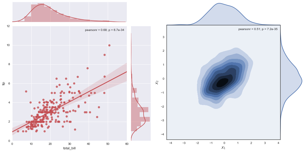
jointplot 主要是用于绘制二元变量分布图。例如，我们探寻 sepal_length 和 sepal_width 二元特征变量之间的关系。

In [21]:

sns.jointplot(x="sepal_length", y="sepal_width", data=iris)
/opt/conda/lib/python3.6/site-packages/scipy/stats/stats.py:1713: FutureWarning: Using a non-tuple sequence for multidimensional indexing is deprecated; use `arr[tuple(seq)]` instead of `arr[seq]`. In the future this will be interpreted as an array index, `arr[np.array(seq)]`, which will result either in an error or a different result.
  return np.add.reduce(sorted[indexer] * weights, axis=axis) / sumval

Out[21]:

<seaborn.axisgrid.JointGrid at 0x7f9c18a3b588>

jointplot 并不是一个 Figure-level 接口，但其支持 kind= 参数指定绘制出不同样式的分布图。例如，绘制出核密度估计对比图。

In [22]:

sns.jointplot(x="sepal_length", y="sepal_width", data=iris, kind="kde")
/opt/conda/lib/python3.6/site-packages/scipy/stats/stats.py:1713: FutureWarning: Using a non-tuple sequence for multidimensional indexing is deprecated; use `arr[tuple(seq)]` instead of `arr[seq]`. In the future this will be interpreted as an array index, `arr[np.array(seq)]`, which will result either in an error or a different result.
  return np.add.reduce(sorted[indexer] * weights, axis=axis) / sumval

Out[22]:

<seaborn.axisgrid.JointGrid at 0x7f9c18afd748>

六边形计数图：

In [23]:

sns.jointplot(x="sepal_length", y="sepal_width", data=iris, kind="hex")
/opt/conda/lib/python3.6/site-packages/scipy/stats/stats.py:1713: FutureWarning: Using a non-tuple sequence for multidimensional indexing is deprecated; use `arr[tuple(seq)]` instead of `arr[seq]`. In the future this will be interpreted as an array index, `arr[np.array(seq)]`, which will result either in an error or a different result.
  return np.add.reduce(sorted[indexer] * weights, axis=axis) / sumval

Out[23]:

<seaborn.axisgrid.JointGrid at 0x7f9c187ec160>

回归拟合图：

Markdown Code

In [24]:

sns.jointplot(x="sepal_length", y="sepal_width", data=iris, kind="reg")
/opt/conda/lib/python3.6/site-packages/scipy/stats/stats.py:1713: FutureWarning: Using a non-tuple sequence for multidimensional indexing is deprecated; use `arr[tuple(seq)]` instead of `arr[seq]`. In the future this will be interpreted as an array index, `arr[np.array(seq)]`, which will result either in an error or a different result.
  return np.add.reduce(sorted[indexer] * weights, axis=axis) / sumval

Out[24]:

<seaborn.axisgrid.JointGrid at 0x7f9c18695a90>

最后要介绍的 pairplot 更加强大，其支持一次性将数据集中的特征变量两两对比绘图。默认情况下，对角线上是单变量分布图，而其他则是二元变量分布图。

sns.pairplot(iris)

此时，我们引入第三维度 hue="species" 会更加直观。

In [26]:

sns.pairplot(iris, hue="species")
/opt/conda/lib/python3.6/site-packages/scipy/stats/stats.py:1713: FutureWarning: Using a non-tuple sequence for multidimensional indexing is deprecated; use `arr[tuple(seq)]` instead of `arr[seq]`. In the future this will be interpreted as an array index, `arr[np.array(seq)]`, which will result either in an error or a different result.
  return np.add.reduce(sorted[indexer] * weights, axis=axis) / sumval

Out[26]:

<seaborn.axisgrid.PairGrid at 0x7f9c17df9d30>

回归图

接下来，我们继续介绍回归图，回归图的绘制函数主要有：lmplot 和 regplot。

regplot 绘制回归图时，只需要指定自变量和因变量即可，regplot 会自动完成线性回归拟合。

In [27]:

sns.regplot(x="sepal_length", y="sepal_width", data=iris)
/opt/conda/lib/python3.6/site-packages/scipy/stats/stats.py:1713: FutureWarning: Using a non-tuple sequence for multidimensional indexing is deprecated; use `arr[tuple(seq)]` instead of `arr[seq]`. In the future this will be interpreted as an array index, `arr[np.array(seq)]`, which will result either in an error or a different result.
  return np.add.reduce(sorted[indexer] * weights, axis=axis) / sumval

Out[27]:

<matplotlib.axes._subplots.AxesSubplot at 0x7f9c1599f6d8>

lmplot 同样是用于绘制回归图，但 lmplot 支持引入第三维度进行对比，例如我们设置 hue="species"。

In [28]:

sns.lmplot(x="sepal_length", y="sepal_width", hue="species", data=iris)
/opt/conda/lib/python3.6/site-packages/scipy/stats/stats.py:1713: FutureWarning: Using a non-tuple sequence for multidimensional indexing is deprecated; use `arr[tuple(seq)]` instead of `arr[seq]`. In the future this will be interpreted as an array index, `arr[np.array(seq)]`, which will result either in an error or a different result.
  return np.add.reduce(sorted[indexer] * weights, axis=axis) / sumval

Out[28]:

<seaborn.axisgrid.FacetGrid at 0x7f9c15e72128>

矩阵图

矩阵图中最常用的就只有 2 个，分别是：heatmap 和 clustermap。

意如其名，heatmap 主要用于绘制热力图。

In [30]:

import numpy as np
np.random.rand(10, 10)

Out[30]:

array([[0.85051983, 0.9145423 , 0.89605792, 0.84944746, 0.74922001,
        0.59267835, 0.99805919, 0.88512193, 0.18599971, 0.56091577],
       [0.12095684, 0.30479607, 0.53430332, 0.62471811, 0.07870098,
        0.13805072, 0.54274945, 0.46251131, 0.56069078, 0.59748567],
       [0.28303197, 0.69632979, 0.26259067, 0.63326556, 0.57107115,
        0.63293859, 0.77295574, 0.40724877, 0.81035974, 0.98412015],
       [0.05975263, 0.33554998, 0.20854645, 0.82509167, 0.12307461,
        0.30298532, 0.63568743, 0.39235473, 0.87438662, 0.67004286],
       [0.68944156, 0.23142135, 0.6135272 , 0.69899901, 0.61543886,
        0.3168536 , 0.57242343, 0.64399907, 0.69877749, 0.64719762],
       [0.93140372, 0.03484852, 0.36875804, 0.16963992, 0.96815741,
        0.8351055 , 0.42740685, 0.23946128, 0.67959917, 0.77029159],
       [0.60736476, 0.33048877, 0.8547361 , 0.37974516, 0.549283  ,
        0.34862862, 0.68027605, 0.50320754, 0.83920003, 0.42048693],
       [0.20869218, 0.59268993, 0.46706104, 0.80358892, 0.31294391,
        0.7570544 , 0.78524166, 0.95219275, 0.50458226, 0.22291758],
       [0.261565  , 0.81460553, 0.70921769, 0.47632015, 0.53507553,
        0.76845005, 0.80753648, 0.5742287 , 0.03967442, 0.44808245],
       [0.50169779, 0.12192067, 0.89638983, 0.30201794, 0.8781447 ,
        0.94818895, 0.41379713, 0.29820411, 0.61002424, 0.05129757]])

In [29]:

import numpy as np

sns.heatmap(np.random.rand(10, 10))

Out[29]:

<matplotlib.axes._subplots.AxesSubplot at 0x7f9c15680cf8>

热力图在某些场景下非常实用，例如绘制出变量相关性系数热力图。

除此之外，clustermap 支持绘制 层次聚类 结构图。如下所示，我们先去掉原数据集中最后一个目标列，传入特征数据即可。当然，你需要对层次聚类有所了解，否则很难看明白图像表述的含义。

In [31]:

iris.pop("species")
sns.clustermap(iris)

Out[31]:

<seaborn.matrix.ClusterGrid at 0x7f9c1454b7b8>

如果你浏览官方文档，就会发现 Seaborn 中还存在大量已大些字母开始的类，例如 JointGrid，PairGrid 等。实际上这些类只是其对应小写字母的函数 jointplot，pairplot 的进一步封装。当然，二者可能稍有不同，但并没有本质的区别。

除此之外， Seaborn 官方文档 中还有关于 样式控制 和 色彩自定义 等一些辅助组件的介绍。对于这些 API 的应用没有太大的难点，重点需要勤于练习。

课后习题

请使用 Seaborn 对示例数据集 tips = sns.load_dataset("tips") 进行数据可视化探索。

实验总结

本章节对 Seaborn 的用法进行了简单的介绍。这里需要说明一下 Seaborn 和 Matplotlib 之间的关系，Seaborn 并不是为了替代 Matplotlib，而应当被看作是 Matplotlib 的补充。对于 Matplotlib 而言，它具有高度自定义属性，可以实现任何你想要的效果。而 Seaborn 非常简单快捷，几行代码就可以画出还不赖的图形。总之，Matplotlib 擅长于纯粹的绘图，而 Seaborn 则多用于数据可视化探索。

继续学习